注釈

Go to the end to download the full example code.

Cyclic Analysis#

This example creates a bladed disc using parametric geometry of a cyclic sector and then runs a modal analysis on that cyclic sector. We then post-process the results using the legacy MAPDL reader and finally generate another cyclic model using our parametric modeler.

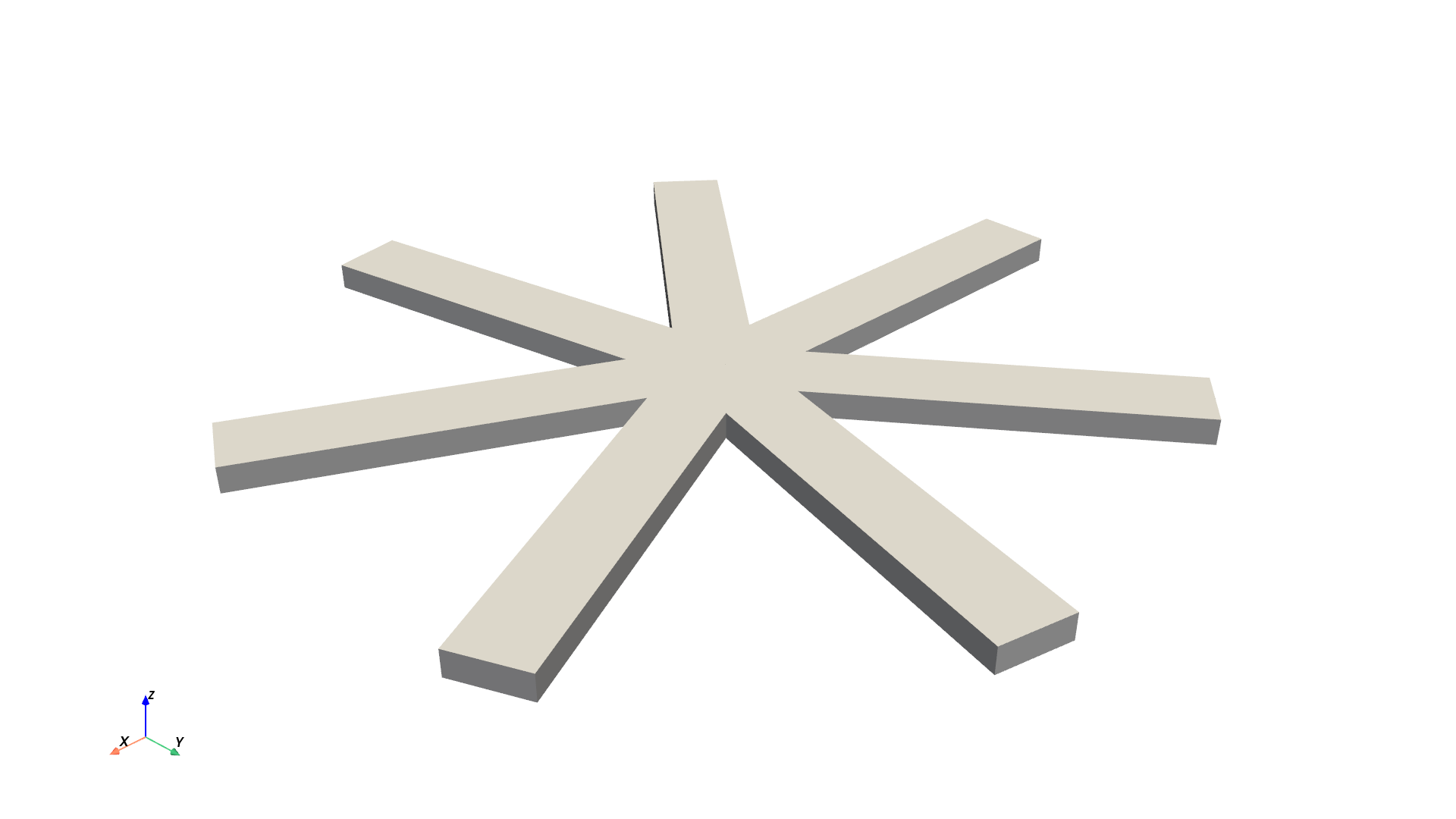
Our first task is to create a simple cyclic model with 7 sectors.

First, start MAPDL as a service.

import numpy as np
import pyvista as pv

from ansys.mapdl.core import launch_mapdl

mapdl = launch_mapdl()

Create the Cyclic Sector#

Create a single "sector" of our cyclic model.

def gen_sector(mapdl, sectors):
    """Generate a single sector within MAPDL."""

    # thickness
    thickness = 0.003  # meters
    arc_end = 2 * np.pi / sectors
    arc_cent = arc_end / 2

    # radius
    rad = 0.01  # M
    arc = pv.CircularArc(
        [rad, 0, 0],
        [np.cos(arc_end) * rad, np.sin(arc_end) * rad, 0],
        [0, 0, 0],
    )

    # interior circle
    kp_begin = [rad, 0, 0]
    kp_end = [np.cos(arc_end) * rad, np.sin(arc_end) * rad, 0]
    kp_center = [0, 0, 0]

    # exterior circle in (M)
    out_rad = 5.2e-2

    # solve for angle to get same arc.length at the end
    cent_ang = arc.length / out_rad / 2

    # interior circle
    kp_beg_outer = [
        np.cos(arc_cent - cent_ang) * out_rad,
        np.sin(arc_cent - cent_ang) * out_rad,
        0,
    ]
    kp_end_outer = [
        np.cos(arc_cent + cent_ang) * out_rad,
        np.sin(arc_cent + cent_ang) * out_rad,
        0,
    ]

    mapdl.prep7()
    mapdl.k(0, *kp_center)
    mapdl.k(0, *kp_begin)
    mapdl.k(0, *kp_end)
    mapdl.k(0, *kp_beg_outer)
    mapdl.k(0, *kp_end_outer)

    # inner arc
    mapdl.l(1, 2)  # left line
    mapdl.l(1, 3)  # right line
    lnum_inter = mapdl.l(2, 3)  # internal line
    mapdl.al("all")

    # outer "blade"
    lnum = [lnum_inter, mapdl.l(4, 5), mapdl.l(2, 4), mapdl.l(3, 5)]
    mapdl.al(*lnum)

    # extrude the model in the Z direction by ``thickness``
    mapdl.vext("all", dz=thickness)


# generate a single sector of a 7 sector model
sectors = 7
gen_sector(mapdl, sectors)

# Volume plot
mapdl.vplot()

Make the Model Cyclic#

Make the model cyclic by running Mapdl.cyclic()

Note how the number of sectors matches

output = mapdl.cyclic()
print(f"Expected Sectors: {sectors}")
print(output)

Generate the mesh#

Generate the finite element mesh using quadritic hexahedrals, SOLID186.

# element size of 0.01
esize = 0.001

mapdl.et(1, 186)
mapdl.esize(esize)
mapdl.vsweep("all")

# plot the finite element mesh
mapdl.eplot()

Apply Material Properties#

# Define a material (nominal steel in SI)
mapdl.mp("EX", 1, 210e9)  # Elastic moduli in Pa (kg/(m*s**2))
mapdl.mp("DENS", 1, 7800)  # Density in kg/m3
mapdl.mp("NUXY", 1, 0.3)  # Poisson's Ratio

# apply it to all elements
mapdl.emodif("ALL", "MAT", 1)

List the Table of Harmonic Indices#

This is the table of harmonic indices. This table provides the corresponding harmonic index for each cumulative mode.

print("C. Index   Harmonic Index")
for i, hindex in zip(range(result.n_results), result.harmonic_indices):
    print(f"{i:3d}      {hindex:3d}")

Generate an Animation of a Traveling Wave#

Here's the nodal diameter 1 of first bend on our cyclic analysis.

We can get the first mode (generally first bend for a bladed rotor) for nodal diameter 1 with:

mode_num = np.nonzero(result.harmonic_indices == 1)[0][0]

pv.global_theme.background = "w"

_ = result.animate_nodal_displacement(
    11,
    displacement_factor=5e-4,
    movie_filename="traveling_wave11.gif",
    n_frames=30,
    off_screen=True,
    loop=False,
    add_text=False,
    show_scalar_bar=False,
    cmap="jet",
)

And here's 1st torsional for nodal diameter 3.

_ = result.animate_nodal_displacement(
    36,
    displacement_factor=2e-4,
    movie_filename="traveling_wave36.gif",
    n_frames=30,
    off_screen=True,
    loop=False,
    add_text=False,
    show_scalar_bar=False,
    cmap="jet",
)

Parametric Geometry#

Since our geometry creation is scripted, we can create a structure with any number of "sectors". Let's make a more interesting one with 20 sectors.

First, be sure to clear MAPDL so we start from scratch.

mapdl.clear()
mapdl.prep7()

# Generate a single sector of a 20 sector model
gen_sector(mapdl, 20)

# make it cyclic
mapdl.cyclic()

# Mesh it
esize = 0.001
mapdl.et(1, 186)
mapdl.esize(esize)
mapdl.vsweep("all")

# apply materials
mapdl.mp("EX", 1, 210e9)  # Elastic moduli in Pa (kg/(m*s**2))
mapdl.mp("DENS", 1, 7800)  # Density in kg/m3
mapdl.mp("NUXY", 1, 0.3)  # Poisson's Ratio
mapdl.emodif("ALL", "MAT", 1)

# Run the modal analysis
output = mapdl.modal_analysis(nmode=6, freqb=1)

# grab the result object from MAPDL
result = mapdl.result
print(result)

List the Table of Harmonic Indices#

Note how the harmonic indices of these modes goes up to 10, or N/2 where N is the number of sectors.

print("C. Index   Harmonic Index")
for i, hindex in zip(range(result.n_results), result.harmonic_indices):
    print(f"{i:3d}    {hindex:3d}")

Plot First Bend for Nodal Diameter 2#

Note how you can clearly see two nodal lines for this mode shape since it's nodal diameter 2.

result.plot_nodal_displacement(
    12, cpos="xy", cmap="jet", show_scalar_bar=False, add_text=False
)

Animate First Bend for Nodal Diameter 2#

Let's end this example by animating mode 12, which corresponds to first bend for the 2nd nodal diameter of this example model.

_ = result.animate_nodal_displacement(
    12,
    displacement_factor=2e-4,
    movie_filename="traveling_wave12.gif",
    n_frames=30,
    off_screen=True,
    loop=False,
    add_text=False,
    show_scalar_bar=False,
    cmap="jet",
)

Cyclic Analysis#

Create the Cyclic Sector#

Make the Model Cyclic#

Generate the mesh#

Apply Material Properties#

Run the Modal Analysis#

Get the Results of the Cyclic Modal Analysis#

List the Table of Harmonic Indices#

Generate an Animation of a Traveling Wave#

Parametric Geometry#

List the Table of Harmonic Indices#

Plot First Bend for Nodal Diameter 2#

Animate First Bend for Nodal Diameter 2#